Often the true, real-world values of model variables or stocks will not be exactly known. When you build a model, you will use the information available to you to create an estimate for a variable value, but there will always be some degree of uncertainty in this estimate. Sensitivity analysis allows you to rapidly explore the impact of this uncertainty to see how robust your results and findings are to changes in variable values. Sensitivity testing works by carrying out multiple simulations of your model using different initial values. It then aggregates the results of the simulation and presents a concise report on the potential simulation outcomes.

To use sensitivity testing, replace one or more of the values in your model with random variables. For instance if you had a stock where your best estimate for the initial value was 100 and you determined you could model an estimate for the true initial value using a random variable with a standard deviation of 7, you would set the initial value of the stock to RandNormal(100, 7).

The model below demonstrates that. Each run draws a fresh starting value, so the curve does not begin from the same place twice.

You may then run the sensitivity testing analysis algorithm to repeat the simulations many times, each time the value of the stock will take on a different initial value and you may see how the resulting simulation paths change (this is a classic Monte Carlo algorithm).

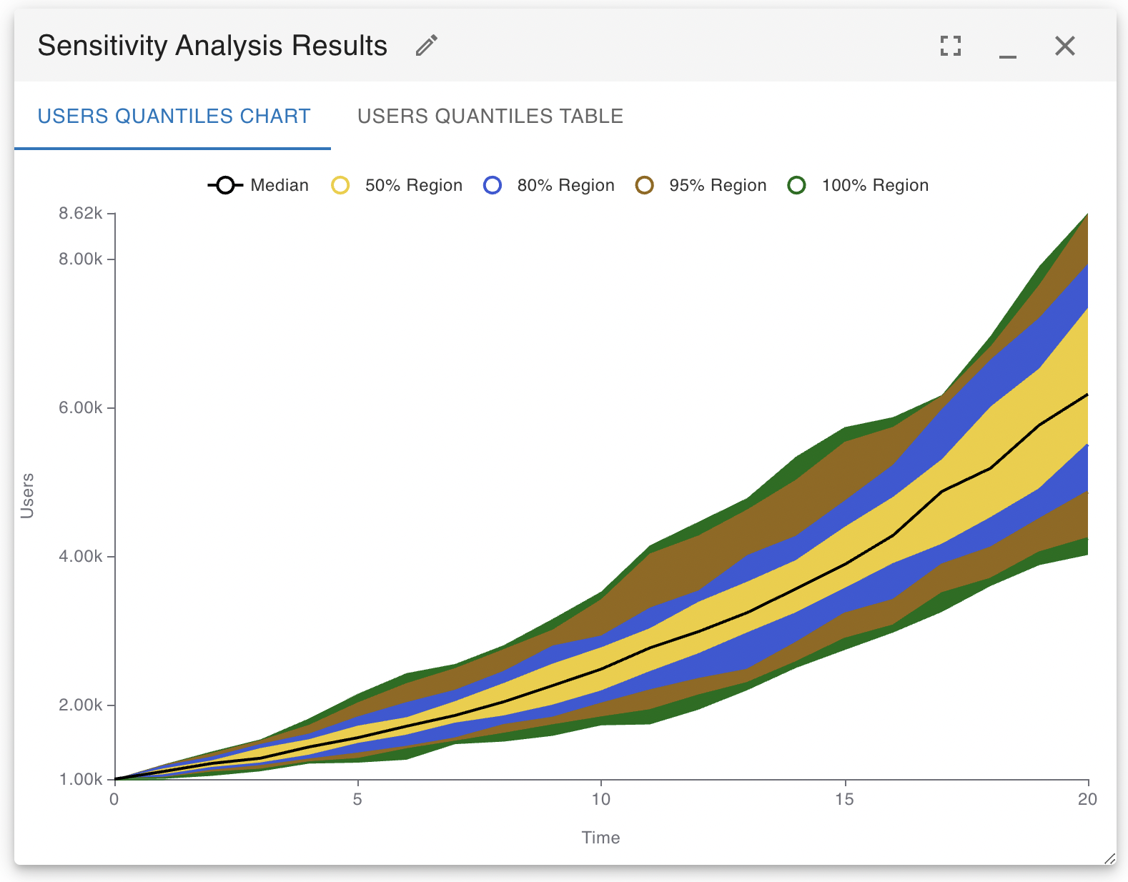
The following is an illustration of the results that can be obtained by carrying out a sensitivity analysis on a different model. The regions that contain the densest 50%, 75%, 95% and 100% of simulation results are clearly marked. A table of these same results is also available for export to Google Sheets, Excel or other analysis programs.

It is important to know that setting the value of a constant variable is not as easy as it is with a stock. If you just place the random function in the variable equation, the variable will take on a different value each time step of each simulation. The editor below plots the value of a variable across a whole simulation, so you can see the value jumping at every step:

If you want to have the variable take on a constant random value for each simulation, you need to use Insight Maker’s Fix function like so. Compare this chart to the one above: the value is drawn once and then held flat for the whole run.

The first parameter to the Fix function is the source value to sample. The second, optional parameter is how often to resample it. Omit it and the value is drawn once at the start of the simulation and held for the whole run, as above. Give it a period and the value is redrawn that often, which is useful for inputs that are constant within a year or a quarter but vary between them:

Each use of Fix in your model keeps its own samples, so two primitives that both call Fix(RandNormal(100, 7)) will hold two different values.